Clinical ISAS Analysis Details
The contents of this webpage describe the details of the ISAS
Analysis using statistical parametric mapping (SPM). The
process is broken down into three phases
- Before you Begin
- Pre-Processing (1.1 - 1.6)
- Setting up the Statistical Model (2.1 - 2.3)
Part 0: Before you Begin
Before you begin analyzing you own patient scans, run ISAS on our
sample patient data.
Once your results
match ours, you can be confident that you are successfuly implementing the process.
Analyze Format
Before beginning the ISAS analysis, verify that the interictal (i.e.
FILENAME_INT.img)
and ictal (i.e.
FILENAME_ICT.img) SPECT scans are in the ANALYZE format
(for more information go to the
Software Setup
page).
Lowercase File Extensions
The extensions of the Analyze format files need to be in
lowercase letters (i.e.
FILENAME.img rather than
FILENAME.IMG).
Note: You can use the DOS rename
command within the image directory (ie.
"rename *.IMG *.img")
or manually rename the files so the extensions
are lowercase.
Radiological Convention
Since we are doing a clinical analysis be sure to set your
SPM default to interpret scans in the Radiologic convention.
Line
28 in the spm_defaults.m file should have the
variable
defaults.analyze.flip set to
1.
Initialize SPM2
Next start SPM2 by typing
spm at the MATLAB prompt.
When SPM starts click
PET and SPECT .
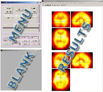
The three SPM windows will be drawn, a menu window,
a blank window for interaction, and a results window.
This interface remains constant throughout the SPM session.

Part 1: Preprocessing the Data
Prior to running the statistical model the images need to be
realigned, normalized, and possibly smoothed and/or masked. We
recommend that you change the color map to HOT for easier viewing
(in the results/graphics window select
Colours->Color Map->HOT).
1.1 Reorient Images:
To view an image click on display in the main SPM window.
The "SPMget" window will pop up and will allow you to browse around
to find the image that you would like to view. You
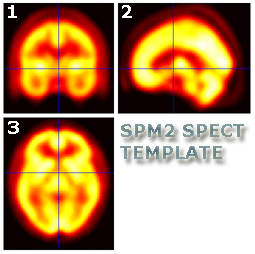
need to reorient the image(s) so it looks like the SPECT template. In
the Graphics Window, you can manipulate the image by changing
the values of pitch, roll and yaw.
Hint: For the sample patient, type in "pi" (which stands for 3.14159265..) as the roll value
to get you image in the correct orientation.
NOTE: The initial SPECT images you see will be dependent
on the scanner you use. Before beginning any analysis, you MUST take a
look through all of your images and make sure everything seems in order.
Take note of any major perfusion deficits or lesions, check the
voxel values to see if they are in the "normal" range, and scan the header
information to make sure everything seems ok.

Re-orientation should result in images that look similar to the SPM SPECT
template located in your
..\spm2\templates folder.
- Frontal view (pane 1) of the brain is upright
- Sagittal view (pane 2) is pointing left
- Transverse view (pane 3) is pointing up
To save this new orientation, click
Reorient Images in the same window.
Then you can apply this change to as many images as you would like.
When SPM asks you for images to reorient, select all of the images to be
reoriented in the same way.
1.2 Set the Crosshairs to the anterior commissure (AC):
Next, you must set the cross hairs in each image so that you
have an equivalent point of reference for all of your images,
namely the
anterior commissure(AC).
Unfortunately there are no short-cuts or ways to automatically
do this and you must do this for every scan. This is actually
one of the only "subjective" steps in your SPM analysis. You don't have
to be exact but the closer you are the better registration you will get
- Click Display and choose your image
(should now be in the correct orientation).
- Click around the image in any of the three planes until you are at the
anterior commissure AC
(you can view the SPECT template to get a feeling for where you should be).
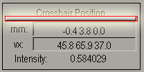
- Once you have found the AC, enter the NEGATIVE of
the x, y, and z coordinates (from the box mm) in the boxes labeled
right forward and up respectively.
For example if the crosshairs position is at -3.1 27.1 4.5 ("mm")
enter the following values in their respective fields:
- right {mm} : 3.1
- forward {mm} : -27.1
- up {mm} : -4.5
- Next click on the horizontal bar under the title of the window,
this should save (register) the new coordinates.

- Click Reorient Images and select the scan
you have been working on.
- Repeat these steps for all the ictal and the interictal scans.
- We recommend that you rotate the pitch, roll, and/or yaw to get the images
to match the template orientations as closely as possible.
1.3 Realigning:
Select Realign in the main SPM window
- Number of Subjects: 1
- Then select the interictal and the ictal scans (in that order)
- Which Option: Coregister and Reslice
- Create What: All images plus mean image
SPM will then create a mean image which will be named
meanFILENAME.img. SPM will also create realigned images for both the
interictal and ictal scans, they will be named
rFILENAME_INT.img and
rFILENAME_ICT.img.
These will be saved in the current directory.
1.4 Spatial Normalization:
This step will warp your realigned images to a standard SPECT
template.
NOTE:
There is an error in the file spm_normalize_ui.m included in SPM2.
A corrected version of this script is available from our scripts downloads section.
Line 513 of this script should read: -90 90 -126 90 -72 108
it did say: -90 90 -126 90 -72 180
This correction needs to be made to ensure that the images have the correct volumes after being normalized to the SPECT template.
Before you can normalize your images you need to set the appropriate defaults.
NOTE:
In previous versions of SPM, if the brain(s) had a large lesion or perfusion defect, the spatial normalization would warp the brain into the lesion area.
In SPM2, the spatial normalization algorithm has improved and normalization keeps the anatomy of the brain intact despite lesions.
For information about creating region masks to deal with specific lesions refer to the
following page.
- Click Defaults in the main SPM window.
- Defaults Area: Spatial Normalization
- Defaults for: Writing Normalized
- Preserve what: Preserve concentrations (the default)
- Bounding Box: Template (this is the only parameter that is not the default)
- Voxel Size: 2x2x2 (default)
- Interpolation Method: Trilinear (default)
- Way to wrap: No wrap (default)
- Click Normalize in the main SPM window.
- Which option?: Determine Parameters and Write Normalized
- Template: SPECT.mnc (located in ..\spm2\templates)
- Source Image Subject 1:
meanFILENAME.img (browse and select the mean image created in the realign step)
- Images to Write Normalized:
Browse and select both the realigned scans rFILENAME_INT.img and rFILENAME_ICT.img
- Source Image Subject 2: click Done
NOTE:
ISAS is a form of clinical analysis in which one patient's scans are compared against the healthy normals database (already normalized).
After the patient's realigned images are chosen, you end the procedure of selecting other scans by clicking done in the SPMget window.
- SPM will then create normalized images named wrFILENAME_INT.img and wrFILENAME_ICT.img
1.5 Masking (optional):
The next step is to mask your image using a brain mask to get rid of any non-brain voxel counts.
Method 1
The simplest masking method (requires downloading ISAS scripts) is to go to
the MATLAB window and type spm_mask_files at the prompt. At the SPMget window which appears select the following
- Select Images to Multiply by a: select both patient scans, order is irrelevant, and click Done (i.e. wrFILENAME_INT.img and wrFILENAME_ICT.img)
- Select Analyze Binary Mask Image: here we choose the brainmask.mnc that SPM2 provides by default (available in the ..\spm2\apriori\ directory)
Matlab will then perform the masking operation and create two more files in the current directory. The masked files are indicated by a concatenated _msk to the end of the filenames (i.e. wrFILENAME_INT_msk.img and wrFILENAME_ICT_msk.img).
Method 2
Another method of creating your own customized mask is by creating a threshold brain mask
by indicating a threshold value below which voxels are eliminated.
- To do this click on imcalc in the main SPM window, and select the image you wish to mask.
- SPM will ask you to label your file and then require you to input an evaluated function.
Enter i1>T (where T is the voxel value threshold below which voxels will be set to 0).
- SPM will then create the output image, and save it (with the name that you specified) in the current directory.
- Once your brain mask has been created, you can follow the same steps as masking using the apriori
brain mask (default brain mask available in the ..\spm2\apriori\ directory)
, but instead of selecting the apriori mask you can select your threshold mask.
Method 3
An alternative, yet more time consuming method is to draw an outline around your scan
using MRIcro. The idea is to display your scan or
mean scan in MRIcro, and then draw a region of interest around the edge of the brain.
This will require you to draw the outline on every slice in at least one plane.
Then, once you have your ROI, you can create a binary image in MRIcro.
For details on how to do this, refer to the MRIcro manual.
1.6 Smoothing:
- Click Smooth in the Main SPM window.
- FWHM:16 16 16
- Choose your masked files (i.e. wrFILENAME_INT_msk.img and wrFILENAME_ICT_msk.img) scans.
SPM will save the smoothed, normalized, and realigned scans as swr*_msk.img
- these will be the scans you will use in the statistical analysis.
Part 2: Statistical Model
Once you've completed the pre-processing steps you are ready to set up your statistical model for your data.
2.1 Change Current Directory
It is important to set the directory where you want to store your statistical analysis files.
For small analysis (clinical) we keep all the preprocessed data and the statistical data in the same folder.
For larger analysis (fMRI studies), you may want to separate your preprocessed data and your
statistical data to organize your files better.
- Click Utils on the main SPM window Select CD
- Choose the folder where you want your results saved (you may need to create a new directory)
by navigating to the desired folder, selecting the small single dot and clicking Done.
2.2 Configure the Model
Now it is time to configure and estimate the statistical model.
- Click PET from the model specification in the SPM menu window.
- Select Multi-Group: Conditions and Covariates
- Number of Groups: 2
- Number of Subjects in Group 1: 1
- Select the smooth-normalized-realigned (and/or masked) image scans (swr*.img) for your patient:
SELECT THE INTERICTAL SCAN FIRST, THEN THE ICTAL SCAN .
NOTE:
The Healthy Normals are added to the model with the Interictal scan followed by the Ictal.
Selecting the Interictal scan (first) and then the Ictal, for the current patient is a key step for ISAS to work properly.
Preserving this order allows for the conditions to be specified only once for the patient and Healthy Normals.
- Condition:0 1 (space in-between, 0 = Interictal, 1 = Ictal)
- Number of Subjects in Group 2: 99 (typing 99 indicates to the spm_spm_ui.m script that the Healthy Normals should be used).
- Number of Covariates: 0
- Number of Nuisance Variables: 0
- Global Normalization: proportional scaling*
- Prop Scan Global Mean: 50
- Threshold Masking: relative
- Analysis Threshold: 0.8
- Global Calculation: mean voxel value**
- Non-sphericity correction: no
*Proportional scaling: a global mean of the image is calculated. This mean includes the zero voxel outside the brain. Then that
mean is divided by 8. The global mean is than recalculated only using voxel with an intensity greater than the old global mean divided by 8.
A proportional scaling factor is determined by dividing 50 ml/min/dl by the new global mean. The image is multiplied by this scaling factor.
The image is then thresholded with a low threshold of 40 (0.8*50) and a high threshold of a really big number.
**Mean Voxel Value: This step refers only to the scaling procedure which occurs before threshold masking (as described above).
Once the model has been setup, click Estimate in the main SPM window.
Select the SPM.mat file
2.3 Set up Contrasts:
Now we will set up the contrasts so that we can compare the statistically significant clusters and voxels
with increases (hyperperfusion) or decreases (hypoperfusion) in cerebral blood flow (CBF).
- Click Results from the Inference panel in the SPM menu window.
- In the contrast manager, select t-contrasts and click on define new contrast
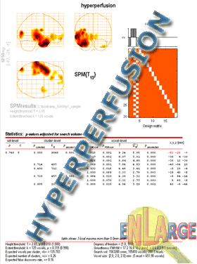
- Enter the title of your contrast: Hyperperfusion (detects CBF increases - positive differences between the scan vs. healthy normals)
- Type 1 1 1 -1 (space delineated) in the contrast box and click submit
- Click define new contrast again to set up the negative contrast
- Enter the title of you second contrast: Hypoperfusion (detects CBF decreases - negative differences between the scan vs. healthy normals)
- Type 1 -1 -1 1 (space delineated) in the contrast box and click submit
2.4 Results
At this point the model has been estimated and the contrasts have been set up.
All that remains is to define significance within the model and to view your results.
- Click the contrast you want to view (i.e. Hyperperfusion) and click done
- Mask results: No
- Title: Hyperperfusion (this title will be displayed on your glass-brain results projection)
- P value adjustment to control: none
- Threshold (p value): 0.01 (you can be more or less stringent i.e. 0.001 or 0.05)
- Extent Threshold: 125 (only include clusters that are made up of 125 or more contiguous voxels)
SPM will spit out the "glass brain" view at this point.

To see the statistics, click Volume from SPM window in the lower left. For easier viewing of scans go to
Colours->ColorMap->Hot.
To save the glass brain results as a JPEG go to
File->Export and
Save as type->JPEG images (*.jpg).
Do this for both the hyper and hypoperfusion contrasts.
Back to Analysis Summary
||
Jump to Top
||
Forward to Displaying Results

